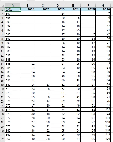
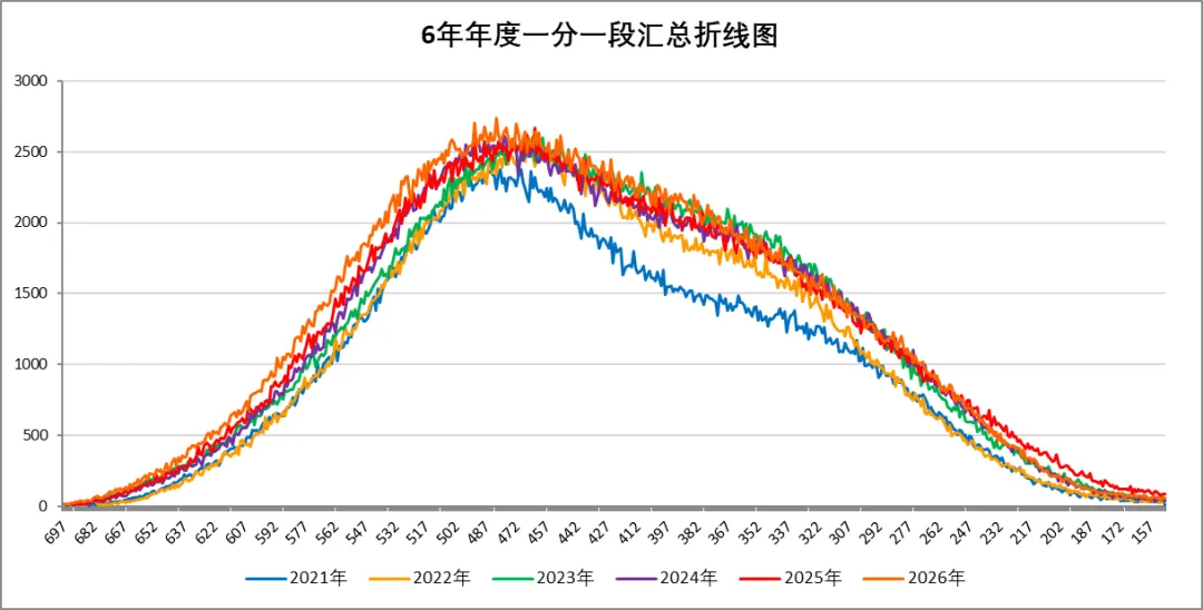
上一篇讲了如何将每年的一分一段表快速生成单年度的柱状图,下面分享一下如何将6年的一分一段表放在一个图表中对比分析。Sub 一键生成6年一分一段折线图表()
Dim 图表宽度 As Double
Dim 图表高度 As Double
Dim 图表垂直间距 As Double
Dim 图表起始左位置 As Double
Dim 图表起始上位置 As Double
Dim 年份配色 As Variant
' 统一图表参数,按需修改
图表宽度 = 480
图表高度 = 240
图表垂直间距 = 0
图表起始左位置 = 900
图表起始上位置 = 10
' 6个年份折线配色 2021/2022/2023/2024/2025/2026
年份配色 = Array(RGB(0, 112, 192), RGB(255, 153, 0), RGB(0, 176, 80), RGB(112, 48, 160), RGB(255, 0, 0), RGB(255, 100, 0))
Dim ws As Worksheet
Dim 最后数据行 As Long
Dim 年份列 As Long
Dim 图表序号 As Integer
Dim 新图表 As ChartObject
Dim 年份值 As String
Dim 数据系列 As Series
Dim arrX As Variant, arrY As Variant
Set ws = ActiveSheet
Application.ScreenUpdating = False
' 清空全部旧图表,下面2行代码进行了注释,实际不运行,如需要清空旧图表,可以取消注释
' On Error Resume Next
' ws.ChartObjects.Delete
On Error GoTo 0
' 读取分数数据最后一行
最后数据行 = ws.Cells(ws.Rows.Count, "A").End(xlUp).Row
If 最后数据行 < 2 Then
MsgBox "未找到A列分数数据!", vbCritical
GoTo 结束程序
End If
Dim 折线图Top As Double
折线图Top = 图表起始上位置 + 图表序号 * (图表高度 + 图表垂直间距)
Set 新图表 = ws.ChartObjects.Add( _
Left:=图表起始左位置, _
Top:=折线图Top, _
Width:=图表宽度, _
Height:=图表高度)
With 新图表.Chart
.ChartType = xlLine
Do While .SeriesCollection.Count > 0
.SeriesCollection(1).Delete
Loop
arrX = ws.Range("A2:A" & 最后数据行).Value
For 年份列 = 2 To 7
年份值 = ws.Cells(1, 年份列).Value
If 年份值 = "" Then GoTo 下一年
arrY = ws.Range(ws.Cells(2, 年份列), ws.Cells(最后数据行, 年份列)).Value
Set 数据系列 = .SeriesCollection.NewSeries
数据系列.Name = 年份值 & "年"
数据系列.XValues = arrX
数据系列.Values = arrY
' 折线线条颜色
数据系列.Format.Line.ForeColor.RGB = 年份配色(年份列 - 2)
数据系列.Format.Line.Weight = 1.5
' 标记点基础设置
' 数据系列.MarkerStyle = xlMarkerStyleCircle
' 数据系列.MarkerSize = 6
' 标记填充色
数据系列.Format.Fill.ForeColor.RGB = 年份配色(年份列 - 2)
' 标记边框色
数据系列.Format.Line.ForeColor.RGB = 年份配色(年份列 - 2)
下一年:
Next 年份列
' 折线图标题
.HasTitle = True
.ChartTitle.Text = "6年年度一分一段汇总折线图"
.ChartTitle.Font.Size = 14
.ChartTitle.Font.Bold = True
' 底部图例
.HasLegend = True
.Legend.Position = xlLegendPositionBottom
.Legend.Font.Size = 9
' 坐标轴与网格
.Axes(xlCategory).TickLabels.Orientation = 45
.Axes(xlCategory).TickLabels.Font.Size = 8
.Axes(xlValue).MinimumScale = 0
.Axes(xlValue).TickLabels.Font.Size = 8
.Axes(xlValue).MajorGridlines.Format.Line.Visible = msoTrue
.Axes(xlValue).MajorGridlines.Format.Line.ForeColor.RGB = RGB(217, 217, 217)
End With
MsgBox "生成完成!" & vbCrLf & "1张6年汇总折线图", vbInformation
结束程序:
Application.ScreenUpdating = True
End Sub
三、操作步骤
- 打开存放一分一段表的 Excel 文件,确认数据格式和文中示例一致;
- 按下快捷键
Alt + F11 打开 VBA 编辑器;
通过这个折线图可以更加直观的对6年的数据进行对比分析,比单独的柱状图更有优势。
 10个月宝宝每天需要喝多少奶粉?

